Predicting Air Quality in Beijing
Academic Project · UCLouvain LELEC2870 · December 2019
Regression models trained on 7 684 records of meteorological and weather data from Beijing (2013–2017) to predict PM2.5 concentration. The project covers feature engineering, correlation and mutual-information selection, PCA extraction, and a benchmark of seven models evaluated with the Bootstrap 632 method.
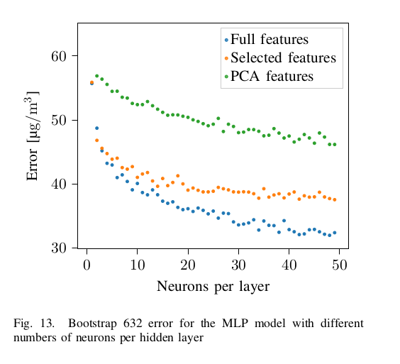
MLP error vs neurons per layer
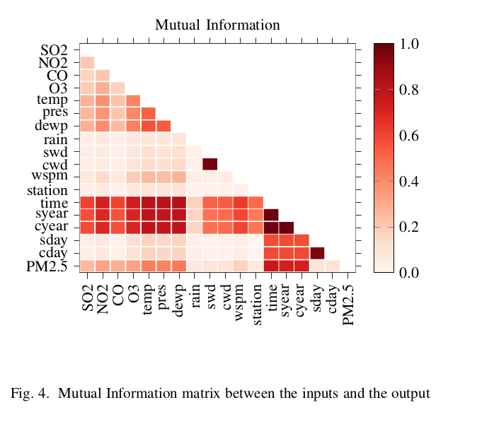
Mutual information matrix
Five-stage ML pipeline
The project follows a rigorous end-to-end pipeline from raw sensor data to validated model selection, emphasising sound error estimation throughout.
Feature engineering
Time encoded cyclically via sin/cos (daily and yearly periods). Wind direction mapped to a wind-rose angle. All 17 features normalized with standard scaling.
Feature selection
Correlation and mutual information used jointly to drop low-relevance features (station, rain, swd…) and redundant ones (temp, pressure, time). Final set: 7 features.
Feature extraction (PCA)
PCA reduces the 17-feature set to principal components. Three components capture the dominant variance (error ≈ 55.5 µg/m³), but non-linear dependencies limit its usefulness here.
Error estimation
Bootstrap 632 method (MLxtend) used throughout — low bias and low variance, making it more reliable than simple k-fold. 10 splits yield σ = 0.255 µg/m³.
Model selection
Seven models trained and cross-compared across all three feature sets. Bootstrap aggregating trees with selected features win at 31.42 µg/m³.
Seven models, three feature sets
Every model is evaluated with the Bootstrap 632 error (µg/m³) on the full feature set, the 7-feature selected set, and the PCA-reduced set. Green bold = lowest error for that model.
Chosen as the final model. Selected features outperform the full set thanks to reduced dimensionality. No overfitting observed up to depth 33.
20 hidden layers · 100 neurons · 300 epochs. Full features win here — the network learns its own feature weighting. PyTorch implementation.
Best depth ≈ 10–11. PCA set overfits at depth 7. Full and selected features plateau without further overfitting.
Selected features strongly outperform full set — high-dimensional Euclidean distance degrades neighbour quality. Best at K = 4.
L1 regularisation sets low-relevance weights to zero. Best at λ = 0.01. Redundant with linear regression given the large training set.
Performance nearly constant for λ ∈ [0.01, 100], then underfits. Best at λ = 0.61.
Validates the feature selection — 7 selected features match the full-set error. PCA performs poorly due to non-linear dependencies.
Key findings
Ensemble methods dominate
Bootstrap aggregating trees halve the error compared to linear baselines (31.42 vs 44.35 µg/m³), confirming that ensemble diversity is the single most impactful lever here.
Feature selection vs extraction
Mutual-information-based selection (7 features) matches or beats the full 17-feature set for all non-neural models. PCA consistently underperforms due to non-linear feature dependencies.
Neural networks need all features
The MLP achieves its lowest error with the full feature set — unlike tree-based models. The network learns its own relevance weighting, making manual selection counterproductive.