Multi-Agent Motion Planning with Military Maps
Graduate Research · UT Austin · Army Research Lab · 2022
Dijkstra-based path planning over multi-layer military terrain meshes with composite cost functions — 3D distance, energy consumption, and terrain valence — extended with coarse-to-fine acceleration for real-time multi-agent routing.
Multi-layer terrain mesh with planned paths
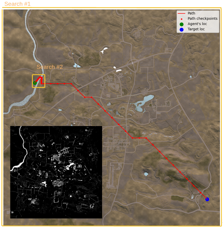
Coarse-to-fine path resolution
Navigating complex military terrain
The core challenge in military path planning is that the terrain isn't uniform — a path that is short in Euclidean distance may cross high-energy ridges or tactically exposed zones. This work builds a graph-based planner that encodes all three dimensions of terrain cost simultaneously.
The Problem
Route multiple agents from start to goal across a military environment represented by overlapping terrain maps — each encoding a different physical constraint. The least-cost path must balance competing objectives.
The Mesh
The terrain is discretized into a graph of nodes. Each node pair has an associated traversal cost based on the underlying map data at that location. The quality of the mesh drives the quality of the path.
The Algorithm
Dijkstra's algorithm finds the globally optimal path in the cost graph. Extended here with multi-objective cost functions and a two-pass coarse-to-fine refinement to reduce computation time without sacrificing path quality at the next checkpoint.
Three maps, one environment
The environment is represented as three independent spatial layers. Each layer contributes a different kind of constraint to the path cost. The planner ingests all three simultaneously to compute composite edge weights across the mesh.
Binary or graded map marking impassable or high-cost terrain — walls, buildings, dense forest, or restricted zones. Edges crossing obstacle cells receive an infinite or very large cost, effectively removing them from the traversable graph.
Hardest constraint: violations are non-negotiable. Acts as a mask before cost computation.
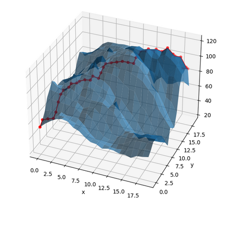
A digital elevation model (DEM) providing height at each grid cell. Used to compute the true 3D Euclidean distance between adjacent nodes — traversing a steep slope costs more than traversing flat ground — and to model the energy required by the agent's dynamics.
Feeds both the distance cost function and the energy cost function. Uphill travel penalized relative to agent weight and grade.
A tactical favorability map: positive values mark covered or advantageous zones (forest, terrain depressions, friendly territory); negative values mark exposed or dangerous areas. Paths through high-valence zones are rewarded with lower cost.
Most interpretable layer for human operators. Encodes domain knowledge not capturable by pure geometry.
How edge costs are computed
Each edge in the graph connects two adjacent mesh nodes. Its traversal cost is assigned by one of several cost functions, or a weighted combination thereof. The choice of cost function determines what kind of path the planner optimizes for.
√(Δx² + Δy² + Δz²)The straight-line distance between two nodes in 3D space, accounting for elevation change. The fundamental baseline cost — a path that is short in 2D may be much longer in 3D when crossing a ridge.
f(m, grade, velocity)Models the mechanical work required for the agent to traverse the edge based on its mass, the slope angle derived from the elevation map, and a nominal velocity. Steep uphill segments are significantly penalized.
−valence(node)Subtracts the valence score of the traversed cell from the edge cost, making tactically favorable zones cheaper to cross. Negative valence (exposed terrain) increases cost.
α·dist + β·energy + γ·valenceA linear combination of the three primary cost functions. The weights α, β, γ are mission parameters set by the operator, allowing a continuous tradeoff between shortest path, minimum energy, and tactical safety.
Coarse-to-fine path planning
Dijkstra on a full-resolution mesh is exact but slow. For real-time applications, a two-pass strategy trades a small amount of global accuracy for a large reduction in computation time — while keeping the immediately-executed portion of the path at full resolution.
Run Dijkstra over a downsampled mesh at low resolution. The result is a sequence of coarse waypoints — checkpoints — that define the gross shape of the optimal route from start to goal.
Run Dijkstra again at full resolution, but only between the agent's current position and the first coarse checkpoint. The agent executes this precise path while the coarse planner already knows the global direction.
Why this works
Routing multiple agents simultaneously
The planner supports N independent agents, each solving its own start-to-goal problem on the same shared terrain. Agents run separate Dijkstra instances over the same cost graph, allowing parallel deployment with independent route optimization.
Each agent computes its own optimal path. Routes may overlap or diverge depending on each agent's start, goal, and mission cost weights.
Different agents can have different α, β, γ weights — a heavy vehicle optimizes for energy; a scout optimizes for valence (concealment).
All agents query the same obstacle, elevation, and valence layers. Terrain updates (e.g., a newly detected obstacle) propagate to all agents' next planning pass.
The coarse-to-fine strategy becomes especially valuable with many agents: the coarse pass is the same regardless of agent count; only the fine pass scales linearly with N.
Proprietary Research
Unlike my other projects, additional details (including the source code) for this research cannot be shared publicly due to a non-disclosure agreement (NDA) signed with the Army Research Lab.